Let’s introduce the final essential categorical concept, the natural transformation. This is an
extremely important concept, I believe Mac Lane has said that he defined the notion of category so
that he could make precise a functor, and he defined a functor to make precise the notion of a
natural transformation.
Definition 1.1.Given two functors \(F\) and \(G\) from \(C\) to \(D\), a natural transformation \(\eta \) from \(F\) to
\(G\) is for each object \(x\) of \(C\), an arrow \(\eta _x\) from \(Fx\) to \(Gx\) such that the following diagram commutes for all
\(x,y,f\):
We write \(\eta : F \Rightarrow G\) to denote a natural transformation.
Natural transformation is a wonderful way of formalizing an intuitive sense of natural. For
example, if \(V\) is a vector space over a field \(F\), there is a dual vector space \(V^*\) which is the vector space of
linear maps from \(V\) to \(F\). Perhaps you know that if \(V\) is finite dimensional, it is isomorphic to its dual.
However these aren’t canonically isomorphic: in order to make an isomorphism, you have to
choose a basis and then identify them. Natural transformation makes precise when this
is canonical. For example, if \(\Vect _F\) is the category of F-vector spaces, then \((-)^*\), the dual, is a
contravariant functor from \(\Vect _F\) to itself. On arrows, \((-)^*\) does the same thing as the \(\Hom \) functor \(C(-,F)\). We
can compose \((-)^*\) with itself to get the covariant double dual functor \((-)^{**}\). If \(f\) is a map from \(V\)
to \(W\), then the double dual makes a map from \(V^{**}\) to \(W^{**}\) as follows: given a map \(g\) that takes
maps \(h\) from \(V\) to \(F\) to \(F\), we get the map \(f^{**}(g)\) that takes maps \(k:V\to F\) to \(g(k\circ f)\). We can define a natural
transformation \(\eta \) from \(1_{\Vect _F}\) to the double dual \((-)^{**}\): given \(v \in V\), we send it to the element of \(V^{**}\) that takes an
element of \(V^{*}\), and evaluates it at \(v\). This is an isomorphism if the vector space is finite
dimension, and note that it is canonical: there was no need to make any choices. Then,
we should expect this collection of maps \(\eta _V, V \in \Vect _F\) to be a natural transformation. And indeed
it is, as one can check by following an element around the diagram that we want to
commute:
Lets follow around an element \(v \in V\):
Another example is the abelianization. Given a group \(G\), we can define a subgroup called the
commutator subgroup \([G,G] = \{aba^{-1}b^{-1}| a,b\in G\}\). The abelianization of \(G\) is the group \(G/[G,G]\). This is a functor as if \(f: G \to H\) is a
homomorphism, we can compose with the projection \(H \to H/[H,H]\) to get a map \(G \to H/[H,H]\). \([G,G]\) is in the kernel of
this map, so we get then a map \(G/[G,G] \to H/[H,H]\). This is the map that the abelianization sends \(f\) to.
Now the projection \(\pi _G: G \to G/[G,G]\) is a natural transformation as the diagram below commutes (by
definition):
As a third example, consider the category \(\omega \) which is the poset category of \(\NN \) with the usual
ordering. Consider a diagram consisting of a sequence of sets \(S_n\) with injective maps from \(S_n \to S_{n+1}\). This can
be thought of as a sequence of sets increasing in size (each containing the previous). Recall that
diagrams are just functors, and in this case, \(\omega \) is the category for which this is a functor (we can call
this functor \(F\). Let \(\widehat{\cup S_i}\) be the constant functor taking \(\omega \) to \(\cup S_i\), and all the arrows to the identity. Then
consider the natural transformation \(\eta : F \Rightarrow \widehat{\cup S_i}\) that sends each \(S_i\) with the subset it corresponds to in the
union. I leave this as an easy exercise to check that this is a natural transformation (draw it!). This
kind of natural transformation is called a cocone (this will be discussed in more depth when we do
(co)limits).
Finally, consider the determinant of a (invertible) matrix, \(\det ^n\). I claim this is a natural
transformation. Consider the two functors from \(\CRing \) to \(\Grp \): one taking \(K\) to \(GL_n(K)\), and the other
taking it to \(K^*\) (check that these are functors). Then \(\det ^n_K\) is for each element of \(\CRing \) a map from \(GL_n(K)\)
to \(K^*\) sending a linear transformation to its determinant. The diagram is the same as
always:
Given two categories \(C, D\), we can form the product category, \(C\times D\) where the objects are pairs of
objects, the arrows are pairs of arrows, and composition is defined as usual.
Now consider the contravariant powerset \(\Set (-,2)\) (2 is a set with two elements, we can view this functor
as \(2^{(-)}\)). As an exercise, try to find all the natural transformations from this functor to itself (this will
come up again in a later lecture).
Definition 1.2.Suppose \(F,G,H\) are functors in \(\Cat (C,D)\). Then if \(\eta :F \Rightarrow G\) and \(\nu :G \Rightarrow H\) are natural transformations, thenwe can form the vertical composite, \(\nu \cdot \eta \), a natural transformation from \(F\) to \(H\), defined by \(\nu \cdot \eta _a = \nu _a \circ \eta _a\).
We can check this is a natural transformation via the following diagram:
This turns \(\Cat (C,D)\) into a category, which we call the functor category. We can write this as \(D^C\). An
isomorphism in \(\Cat (C,D)\) is called a natural isomorphism. Alternatively, it is a natural transformation \(\eta \)
where each \(\eta _a\) is an isomorphism.
I use the word vertical composite, because there is also a horizontal composite. It can be seen as
follows:
Given the diagram below, we would like to create a natural transformation \(\nu \eta : F' \circ F \Rightarrow G' \circ G\) sometimes written \(\nu \circ \eta \).
We can do this by considering the following diagram:
This commutes as \(\nu \) is natural for \(\eta _a\). This suggests the following definition:
Definition 1.3.Suppose \(F,G,F',G',\eta ,\nu \) are as above, we can form the horizontal composite \(\nu \eta :F' \circ F \to G'\circ G\) so that \((\nu \eta )_a = \nu _{Ga} \circ F'\eta _a = G'\eta _a \circ \nu _{Fa}\).
It remains to check this is a natural transformation, but this should be obvious if you draw the
appropriate diagram (for a natural transformation). If \(F: C \to D\), \(G,H: D \to E\) are functors and \(\eta : G \Rightarrow H\) a natural transformation
then the natural transformation \(\eta F\) denotes the horizontal composite \(\eta 1_F\), and similarly if \(J: E \to X\) is a functor,
then \(J\eta \) denotes \(1_J\eta \).
Horizontal composites and vertical composites are related through the interchange law, which
says \((\tau \eta )\cdot (\tau '\eta ')=(\tau \cdot \tau ')(\eta \cdot \eta ')\). It can be described as the diagram below:
We can prove it using the diagram below. Let \(\eta ': F \Rightarrow G, \eta : G \Rightarrow H, \tau ': F' \Rightarrow G', \tau : G' \Rightarrow H'\) in the figure above.
The path on the top is the natural transformation \((\tau \cdot \tau ')(\eta \cdot \eta ')\), and the path on the bottom is \((\tau \eta )\cdot (\tau '\eta ')\). The middle
rectangle commutes as \(\tau '\) is a natural transformation.
As a final note, there is an analogy between natural transformations and homotopies.
If \(X\) and \(Y\) are topological spaces, and \(f\) and \(g\) are maps (continuous, as always) from \(X\) to \(Y\), a homotopy
from \(f\) to \(g\) is a map from \(X \times [0,1]\) to \(Y\) that at \(0\) restricts to \(f\) and at \(1\) restricts to \(g\). The definition
of a natural transformation can be presented analogously: Let \(2\) be the category with \(2\)
objects, called \(0\) and \(1\) and one non identity arrow from 0 to 1 (we can say the arrow
category, as this is the category that represents the diagram consisting of a generic
arrow).
If \(C\) and \(D\) are categories, and \(F\) and \(G\) are functors from \(C\) to \(D\), a natural transformation
is a functor from \(F\) to \(G\) is a functor from \(C\times 2\) to \(D\) that on \(0\) restricts to \(F\) and on \(1\) restricts to
\(G\).
Check that these two definitions of natural transformations are equivalent and note the
similarity with homotopies. In a way, a natural transformation is categorification of
homotopy.
Finally let’s end with an interesting non-example. Let \(\FinSet _g\) be the category of finite sets and
bijections between them. Consider two functors to Set, the first, \(\Aut \), takes \(X\) to the set of bijections
from \(X\) to itself, on maps, it takes \(f: X \to Y\) to the function that takes \(\phi :X \to X\) to \(f \circ \phi \circ f^{-1}: Y \to Y\). The second, \(\Ord \), takes \(X\) to the set of
total orders on \(X\), and on maps takes \(f\) to the total order on \(Y\) induced by the bijection. These two
functors send isomorphic objects to isomorphic sets, but are not naturally isomorphic: in
fact, there isn’t even a natural transformation between them! For, let’s consider \(f\), the
nontrivial bijection from a set \(\{a,b\}\) to itself. If there was a natural transformation, we would
have
\(\Aut (f)\)is the identity, but \(Ff\) is not, so this diagram cannot commute.
The fact that this bijection is not natural has an interesting interpretation in the context of a
combinatorics problem. In particular, let’s count the number of trees on a set of \(n\) elements, which
we’ll call \(T_n\). Let \(|\cdot |\) denote cardinality of a set. Consider the product \(T_n \times n \times n\), consisting of a tree on the set \(n\),
as well as a head and a tail (shown in Fig 2).
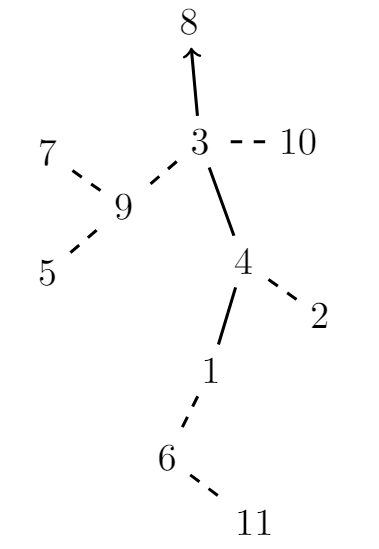
Figure 1:A tree, on 11 elements, with a skeleton, indicated by the bold lines, is determined
by the total ordering on the skeleton and the trees coming out of each point on the skeleton.
Note that since there is a unique path between any two points in a tree, we can draw an arrow
from the tail to the head, yielding a total ordering on a subset of 1 to n, ie. a skeleton, as well as
trees coming out of each point. Note that the skeleton and the trees coming out of each point
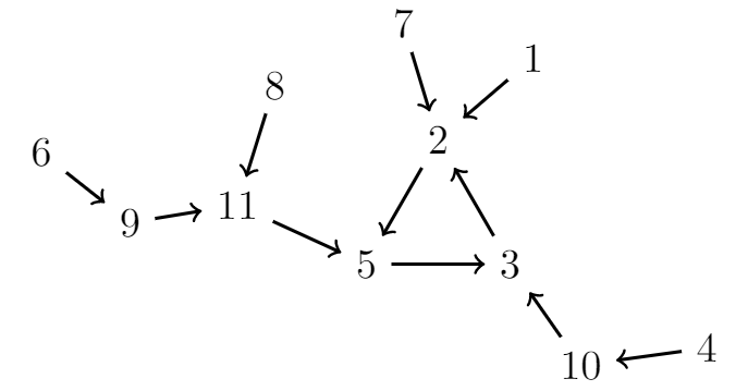
completely determine \(T_n \times n \times n\). Then as total orders are in bijections with permutations, we can consider
the set of permutations with trees coming out of them, a typical example in the figure
below:
Figure 2:A permutation on 2, 3, and 5 with trees coming out of it.
These are in bijection with functions from the set of n elements to itself, as a function
determines such a tree by writing where everything goes, which eventually (after applying the
function enough times) determines the cycles and the trees coming out of them. Thus \(T_n \times n \times n\) is in
bijection with the set of functions from \(\{1,... ,n\}\) to itself, which is \(n^n\). Thus \(|T_n| = n^{n-2}\) (This is known as Cayley’s
Theorem). Perhaps the reason this proof does something nontrivial is because it used this bijection
which was unnatural.


![G G ∕[G, G ]
πGπH H H ∕ [H, H ]](Natural_Transformations3x.svg)